srf.BackToVMR

After creating/morphing a surface, it is often helpful to visualize in a voxel-based representation where the vertices (and triangular planes inbetween) are located in space. This method allows to do so by creating either a 1mm- or a 0.5mm- resolution dataset which can then be sampled (or merged with a VMR, the original purpose).

You simply need the surface object you wish to visualize in voxel space.

 SRF::BackToVMR  - back-project vertices to VMR space
 
 FORMAT:       [srf = ] srf.BackToVMR([opts])
 
 Input fields:
 
       opts        optional settings
        .fillmode  either of {'nearest'} or 'linear'
        .nfrom     Vertex + from * Normal (default: -0.25)
        .nstep     step along normal(default: 0.5)
        .nto       Vertex + to * Normal (default: nfrom + nstep)
        .res       VMR resolution, either of {1} or 0.5
        .triovsmp  triangular oversampling factor (default: 2)
 
 Output fields:
 
       srf         SRF object with VertexVMRData set accordingly

Options are passed as a struct. In the default case, a clearly visible layer (between one and two voxels usually) will be drawn. Depending on the mesh resolution, you might want to increase the triangle oversampling factor, for instance.

The fillmode determines how the VMR values will be filled. For nearest, each determined coordinate (vertex + multiplied normal vector, potentially triangular subsampled), will be rounded off and the resulting voxel will be set to a fixed value. For linear, the determined position will be distributed to all 8 adjacent voxel coordinates (box corners), according to the proximity of the determined position.

These three parameters determine how many sampling passes are performed and how far along the normal vector the sampling occurs. This is helpful if you wish to fill a thicker layer in voxel space, e.g. for creating a mask that covers more space.

In case you are working in 0.5mm resolution (BrainVoyager's advanced segmentation), you can switch to that resolution (in which case you might want to increase the triangular oversampling factor as well, see below!).

This parameter sets the triangular oversampling factor. The higher this value is, the more points within each triangle will be sampled. For example, with an oversampling factor of 5, each side of the triangle is split 5-fold and the meeting points of the parallel lines will be sampled.

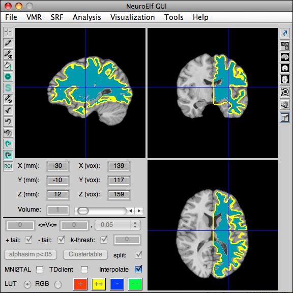
This image represents the ICBM normalized left-hemisphere (radiological convention!) display of the colin_LH_ICBMnorm.srf file overlaid on the colin_brain_ICBMnorm.vmr (using a 6-times oversampling in triangles to cope with differences in triangle size). The interior has then been flood-filled with a code of 240 for voxels in the range 150 through 225.