For many experimental tasks (e.g. subjects follwing a set of specific but differing instructions), it is often helpful to collect secondary physiological measurements, such as heart-rate over time (both as a manipulation check but also as potential candidates for mediation analysis). The data processing can be rather complicated, and a function to automatize the actual detection of heart beats in the ECG data is helpful.

The raw signal (ECG channel recording) must be available in a Matlab variable. For the purpose of this manual, this variable is called data. The xff IO reading class now supports reading the following formats:

• ACQ (up until version ⇐ 3.9.7)
• TXT (use object = xff('*.ntt'); or object = xff(filename, 'ntt'); to read!)

and further formats might be added based on request and urgency.

In case the data is in a different format, you must ensure to first convert into one of the formats above or into a MAT file, which then can be read used like this:

heartbeats_readmat.m

% load a mat file (e.g. an ACQ->MAT converted file)
load HPS1344_session1_ECG.mat;
 
% create new NTT (used for methods on data!)
ntt = xff('new:ntt');
 
% store data from mat file in ntt
ntt.Data = data;

Output of help heartbeats:

  heartbeats  - detect heart beats and frequency in physio data
 
  FORMAT:       [bp, bs, bf, bv, cp, wgd, wd, hrv] = heartbeats(sig [, opts])
 
  Input fields:
 
        sig         Sx1 numeric signal
        opts        optional settings
         .badt      t-threshold for detecing irregularity (default: 25)
         .bppre     pre-defined positions (no detection, only inspection)
         .calc      preprocessing calculcation, one of
                    {'none'} - don't to anything (default)
                    {'absdiff'} - use abs(diff(data))
                        if .detlength is not given, will be set to 0.02
                        if .skewdt is not given, will be set to 0.1
                    {'diffsq'} - square the diff of the data
                        if .detlength is not given, will be set to 0.01
                        if .skewdt is not given, will be set to 0.05
                    {'fourthz'} - fourth power of the z-transformed data
                        if .detlength is not given, will be set to 0.02
                        if .skewdt is not given, will be set to 0.04
                    {'squarez'} - square the z-transformed data
                        if .detlength is not given, will be set to 0.03
                        if .skewdt is not given, will be set to 0.1
                    {'thirdz'} - third power of the abs z-transformed data
                        if .detlength is not given, will be set to 0.02
                        if .skewdt is not given, will be set to 0.06
         .cleanup   interactive cleanup (default: false)
         .detlength detection length threshold in seconds (default: 0.05)
         .freq      data frequency in Hz (default: 1000)
         .pflength  pre-filter length in seconds (default: 0.025)
         .pfreps    pre-filter repetitions (default: 2)
         .plot      plot mean +/- std estimate of signal (default: false)
         .plotfreq  samples per second to plot (default: 50)
         .plotwin   plot window size in seconds (default: 6)
         .resfreq   resample data prior to detection (default: [])
         .segsize   segmentation size in seconds (default: 5)
         .segstep   stepping (window shift) in seconds (default: 1)
         .skewdt    skewness detection threshold multiplier (default: 0.5)
         .winsor    winsorizing threshold in std's (default: 3)
 
  Output fields:
 
        bp          beat positions
        bs          beat positions (in seconds)
        bf          frequency estimate for each beat
        bv          values at peak
        cp          estimate of centers of windows (one value less!)
        wgd         guess whether window is good or not
        wd          windowed data (in 100Hz resolution, interpolated)
        hrv         output of computehrv(bp)
 
  Note: this function is still preliminary, other options passed on to
        computehrv (if 8th output is requested), with .hrvrfreq being
        set to .resfreq

Once the data is loaded, the function call is relatively straight forward. For the “first pass”, cleanup should be enabled, as well as plotting the results:

[bp, bs, bf, bv, cp, wgd, wd] = ...
    heartbeats(data, struct('cleanup', true, 'plot', true));

This will perform the following steps (if no pre-defined beat positions are given):

• windowed z-transform (in segment windows with configured stepsize, also works as low-pass filter!)
• windsorizing (cutting off over-large peaks)
• filtering (low-pass, to get rid of very high frequency noise)
• possible skew-flipping (to ensure that peaks always are towards the positive tail of the distribution)
• segment-wise beat detection (maximum value position within each sub-segment where value > mean + 0.5 * skew)
• if not enough beats are found (currently less than 6 per minute overall) the best general fit over the auto-correlation is computed and beats are completely re-estimated

Next, the detected (or provided) beats will be analyzed as follows:

• the robust mean over the distance of beats (heartrate) is computed
• any beat closer together than 1/3 of that distance is removed
• any gap larger than 3 times that distance is automatically filled up (at located within segments)
• each segment surrounding any given beat will be resampled to 101 values (fixed resolution)
• the mean over segments with a suitable length will be taken as the reference
• a t-statistic is computed for how much variance in each of the segments is accounted for (better scaled than r or F)
• all segments below the specified threshold (default t=25) will be marked as irregular

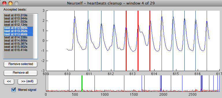
Any of these irregularities (that is to say, places where either the distance between beats is too small or too large or the shape of the detected beat does not match the mean signature) will be displayed, one by one, in a small dialog:

Some info on the controls:

• the larger time course plot shows an excerpt of the provided signal (data) around the detected irregularity
• the smaller time course plot gives the entire signal (noise estimate) along with indicators of irregularities (blue lines) and the current position (green line); this can be used to directly visit a problematic area by clicking into this smaller time course plot
• the list box contains the positions of detected (accepted) beats in the window of the larger time course excerpt
• the buttons below can be used to remove beats from the list and to navigate to the previous or following irregularity
• the checkbox below the buttons switches between raw and filtered timecourse (only available if filtering was performed initially)

The operation is relatively simple:

• to add a beat in the stream, simply press the mouse button close to the desired peak location (which will be determined in a +/- 100ms window around the clicked spot)
• to remove a beat (or several beats), select those in the dropdown box and press the “Remove selected” button
• to remove all beats in the current window, press the “Remove all” button
• once all beats in this window are correct, you can either move backward («) or forward (») in time, or click into the overview timecourse

If no more irregularities remain to be checked (after clicking next, », when the last irregularity was displayed), the dialog will close automatically. If you wish, you can also manually close the dialog (prematurely) to go on to the next stage.

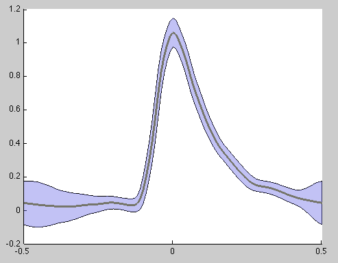
In case the plotting has been enabled, the following two displays appear:

This first figure simply shows a representation of the mean (each window is re-sampled to match a 100-sample window length) and the standard deviation, whereas the X-axes is labeled as phase with the peak being located at 0. This display can be helpful in fine-tuning some of the parameters for the function (e.g. the detection length threshold).

The second figure shows the entire signal over time in a 20Hz sampling (in blue) with the detected heart-rate (which is rescaled to 2.5 + BPM/60) super-imposed to control for flaws in the (initial auto-) detection. This can be done by zooming in on a smaller piece of the signal:

.

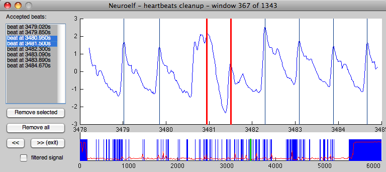
Sometimes, the data is very noisy (like this):

At this point, the function (heartbeats) does not yet have any pre-processing algorithms. After consultation with colleagues, I might decide to add those functions in a future version.

Naturally, it is possible to script this function, save the pre-detected heartbeats (without manual interaction/plotting) and then, at a later time, revisit the inspection (for instance, if several subjects' datasets are to be examined, it usually is preferable to perform the extraction and detection of all datasets prior to engaging in the fine tuning).

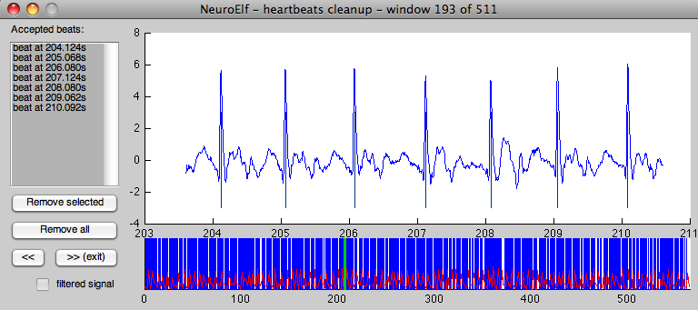
For instance, if the raw signal looks like this

A two-pass detection scheme can be employed:

heartbeats_crisp_detection.m

% first, load the data
data = xff('*.ntt');
 
% then z-transform the third column (in our case) and take the 4th power
pdata = ztrans(data.Data(:, 3)) .^ 4;
 
% pre-detect beats
% since we used the 4th power, the skew detection threshold must be lowered
% and our signal has short spikes, so the detection length threshold also!
bp = heartbeats(pdata, struct( ...
    'skewdt',    0.05, ...
    'detlength', 0.01, ...
    'freq', 500));
 
% then pass this along with the actual signal back in
[bp, bs, bf, bv, cp, wgd, wd] = heartbeats(data.Data(:, 3), struct( ...
    'bppre',   bp, ...
    'cleanup', true, ...
    'freq',    500, ...
    'plot',    true));